[TensorFlow] 기초 개념 및 수행 결과 _ 5. Tensorboard : Graph Visualization 사용하기

import tensorflow as tf

input_data = [[1,5,3,7,8,10,12],

              [5,8,10,3,9,7,1]]

label_data = [[0,0,0,1,0],

              [1,0,0,0,0]]

​

INPUT_SIZE = 7 

HIDDEN_SIZE_1 = 10

HIDDEN_SIZE_2 = 8

CLASSES = 5

x = tf.placeholder(tf.float32, shape = [None, INPUT_SIZE], name="x" )

y = tf.placeholder(tf.float32, shape = [None, CLASSES], name="y" )

tensor_map = {x : input_data, y : label_data}

weight_hidden_1 = tf.Variable( tf.truncated_normal(shape=[INPUT_SIZE, HIDDEN_SIZE_1]) , dtype=tf.float32, name="weight_hidden_1" ) 

bias_hidden_1 = tf.Variable( tf.zeros(shape=[HIDDEN_SIZE_1]) , dtype=tf.float32, name = "bias_hidden_1" )

​

weight_hidden_2 = tf.Variable( tf.truncated_normal(shape=[HIDDEN_SIZE_1, HIDDEN_SIZE_2]) , dtype=tf.float32, name="weight_hidden_2" ) 

bias_hidden_2 = tf.Variable( tf.zeros(shape=[HIDDEN_SIZE_2]) , dtype=tf.float32, name = "bias_hidden_2" )

​

weight_output = tf.Variable( tf.truncated_normal(shape=[HIDDEN_SIZE_2, CLASSES]) , dtype=tf.float32, name="weight_output" ) 

bias_output = tf.Variable( tf.zeros(shape=[CLASSES]) , dtype=tf.float32, name = "bias_output" )

param_list = [weight_hidden_1, bias_hidden_1, weight_hidden_2, bias_hidden_2, weight_output, bias_output ]

saver = tf.train.Saver(param_list)

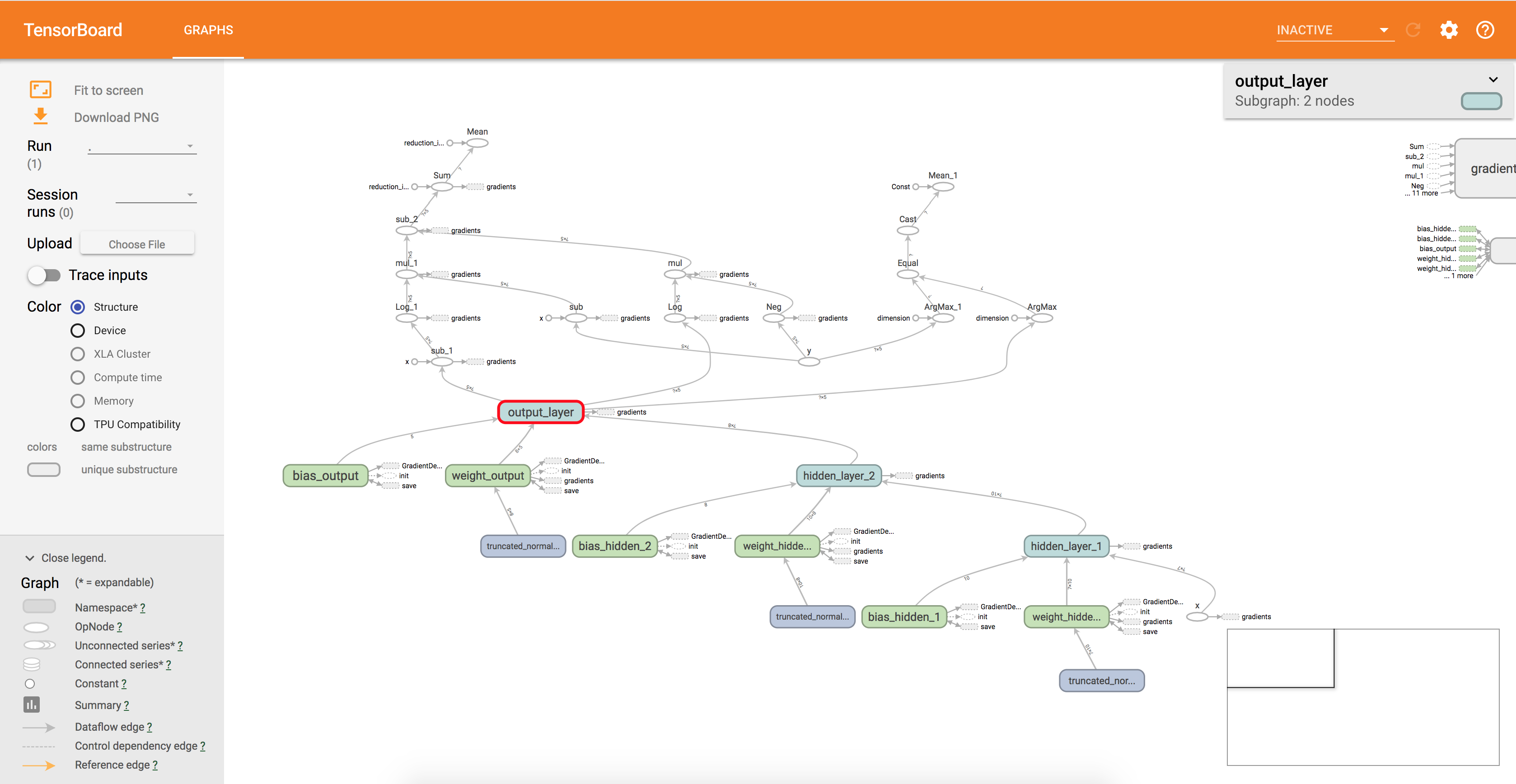
with tf.name_scope('hidden_layer_1') as h1scope:

    hidden_1 = tf.matmul( x , weight_hidden_1 , name="hidden_1" ) + bias_hidden_1

with tf.name_scope('hidden_layer_2') as h2scope:

    hidden_2 = tf.matmul( hidden_1 , weight_hidden_2, name="hidden_2" ) + bias_hidden_2

with tf.name_scope('output_layer') as osscope:

    answer = tf.matmul( hidden_2 , weight_output, name="answer" ) + bias_output

Learning_Rate = 0.05

​

cost_ = -y*tf.log(answer)-(1-y)*tf.log((1-answer))

cost = tf.reduce_sum(cost_, reduction_indices=1)

cost = tf.reduce_mean(cost, reduction_indices=0)

train = tf.train.GradientDescentOptimizer(Learning_Rate).minimize(cost)

​

comp_pred = tf.equal( tf.arg_max(answer, 1), tf.arg_max(y, 1) )

accuracy = tf.reduce_mean(tf.cast(comp_pred, tf.float32))

​

sess = tf.Session()

init = tf.global_variables_initializer()

sess.run(init) 

​

saver.restore(sess, './tensorflow_live.ckpt')

merge = tf.summary.merge_all()

​

for i in range(1000):

    _ , loss, acc = sess.run([train, cost, accuracy], feed_dict = tensor_map)

    if i%100 == 0:

        train_writer = tf.summary.FileWriter('./summaries', sess.graph)

        saver.save(sess, './tensorflow_live.ckpt')

        print ( '---------------' ) 

        print ( 'step    : %f' %  i  )

        print ( 'loss    : %f' % loss)

        print ( 'accuracy: %f' % acc ) 

sess.close()